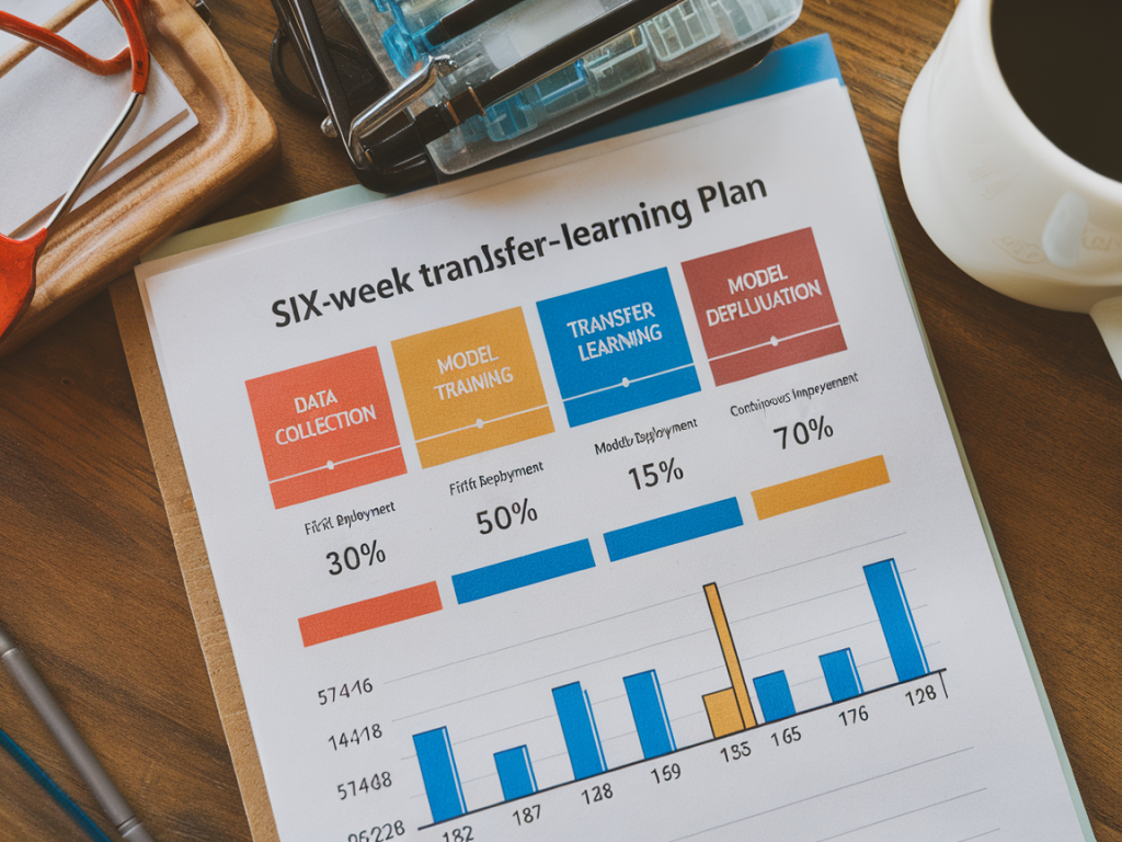
I remember the first time a new product family landed on my desk and the plant asked, "How quickly can we get acceptable inspection performance?" The short answer I gave then — and keep giving now — is: faster than you think, if you structure the transfer‑learning work properly. Below I walk through a pragmatic six‑week plan I use to halve false rejects (Type I errors) when introducing a new product family to an existing vision inspection or anomaly‑detection model.
Why focus on transfer learning for new product families?
When a line introduces a new part, changes in geometry, surface finish, or packaging often cause a spike in false rejects. Training a model from scratch takes time and data. Transfer learning lets us reuse representations learned on the existing product families and adapt them rapidly with far less labelled data. In practice, that means fewer line stoppages, less rework, and faster ramp‑up to stable throughput.
What my goal looks like — measurable and actionable
I always define the desired outcome before touching data or models. For this plan the objective is:
- Reduce false rejects by ~50% versus the baseline during the first four weeks of production.
- Keep false accepts (missed defects) at or below baseline risk — we don't compromise safety or quality for throughput.
- Deploy a validated model into production within six weeks, with an operational monitoring dashboard and an online feedback loop for continuous improvement.
High‑level week‑by‑week roadmap
Below is the practical six‑week schedule I use. It assumes you have an existing vision model, basic MLOps capability (model registry, CI/CD, and a way to collect labelled rejects), and a cross‑functional team: process engineer, data scientist, data engineer, and operations lead.
| Week | Main activities | Deliverable |
|---|---|---|
| Week 1 | Data intake, quick process audit, baseline metrics | Baseline report + prioritized defect types |
| Week 2 | Collect/curate labelled samples, initial transfer training | Adapted model prototype + training logs |
| Week 3 | Active learning loop, focused labelling, hyperparameter tuning | Validated candidate model (offline metrics) |
| Week 4 | Pilot deployment on a single line segment, real‑time monitoring | Pilot results, adjustment plan |
| Week 5 | Scale deployment, integrate operator feedback, threshold calibration | Production model in registry + rollback plan |
| Week 6 | Operationalize monitoring, build continuous learning pipeline | Dashboard, SLA for retraining, and roadmap for further improvement |
Week 1 — rapid audit and baseline
Start by spending half a day on the shop floor and the other half with the data. My checklist for Day 1:
- Capture the current false‑reject rate by defect type and by camera/station.
- Identify process shifts between new and legacy products (lighting, conveyor speed, part orientation).
- Retrieve existing model weights, preprocessing pipeline, and augmentation strategy.
- Confirm where labelled ground truth lives and how operators mark rejects in MES.
This gives you the baseline and helps you prioritize: are cosmetic scratches the main issue, or is it a new material that confuses the model? The more specific your defect taxonomy, the faster you can target the adaptation.
Week 2 — targeted data collection and initial transfer
Transfer learning thrives when you provide a small but representative labelled set. I aim for an initial labelled pool of 200–1,000 images, stratified by defect class and production conditions. Use these guidelines:
- Collect both clean samples and edge‑case rejects — boundary examples are gold for threshold tuning.
- Maintain the same preprocessing pipeline used in production (same cropping, resizing, color normalization).
- Augment cautiously: simulate plausible variations (minor rotations, brightness changes), but avoid unrealistic transforms that introduce label noise.
For model adaptation, I typically freeze early convolutional layers and fine‑tune the later layers and classifier head. If you’re using off‑the‑shelf architectures (ResNet, EfficientNet) or frameworks like PyTorch Lightning or TensorFlow, this step is quick. I also test two approaches in parallel: fine‑tuning and training a small domain‑specific classifier on top of frozen embeddings (cheap and often surprisingly effective).
Week 3 — active learning and validation
After the initial training, use active learning to pull the most informative samples from ongoing production. I deploy a lightweight scoring agent that flags low‑confidence predictions and routes those images to a rapid human review queue. Prioritize labelling:
- Low‑confidence false rejects that operators disagreed with.
- False accepts discovered during QA sampling.
- Boundary conditions identified in Week 1 (e.g., reflections, color shifts).
Validate candidate models on a hold‑out set that simulates production mix. Look beyond accuracy — use precision for rejects (precision = fraction of predicted rejects that are true rejects) and recall for defects you cannot miss. I also plot Receiver Operating Characteristic (ROC) and Precision‑Recall curves to choose thresholds aligned to business risk.
Week 4 — pilot on the line
Piloting in production is where theory meets reality. Deploy the candidate model to a single inspection station in monitoring mode first (scores visible but not flagging parts). This has three benefits:
- Collect real operating data without disrupting the line.
- Observe context features that weren’t captured in the lab (vibrations, extreme lighting).
- Allow operators to build trust via side‑by‑side comparison.
After 48–72 hours of monitoring and a few hundred samples, move to active reject mode with conservative thresholds and back‑stop manual review. Expect to iterate thresholds and minor preprocessing adjustments.
Week 5 — scale out and feedback loops
With a stable pilot, roll the model to additional stations. Key tasks:
- Integrate operator feedback into the labelling queue (a simple mobile app or a MES flag works).
- Automate data capture pipelines to feed the retraining set nightly.
- Document rollback criteria: if false rejects spike > X% over baseline, revert automatically and notify stakeholders.
This week I also formalize the MLOps steps: model versioning (MLflow, DVC, or a model registry), deployment artifacts, and a CI pipeline for retraining and testing.
Week 6 — operationalize monitoring and plan continuous improvement
In week six I focus on durability. Deliverables I hand off include:
- A monitoring dashboard (Grafana or a lightweight custom UI) showing false reject rate, false accept incidents, confidence histograms, and data drift metrics.
- An SLA for retraining cadence (e.g., weekly minor retrain if drift > threshold, full retrain quarterly).
- A documented operator workflow for rapid labelling and escalation of weird cases.
Finally, I schedule a retrospective with stakeholders to capture lessons learned and to set the next goals: further halving false rejects, expanding to other product families, or integrating physics‑based checks alongside vision models.
If you want, I can share a lightweight GitHub template for the training/CI pipeline I use, or a sample dashboard configuration for monitoring. On Ccsdualsnap Co (https://www.ccsdualsnap.co.uk) I also have a companion checklist and a case study showing how we cut false rejects by 60% for an electronics assembly line using this exact cadence.