I recently ran a small but rigorous pilot to prove that a smart patch — a thin, non‑intrusive device that detects cycle start/end and key process states — could cut cycle time by about 20% on a discrete assembly operation. I used a Raspberry Pi as an edge gateway to collect, pre‑process and forward high‑frequency events to our cloud historian, and I focused the analysis on before/after KPI comparisons with clear statistical checks. I’m sharing the approach, the implementation details, and the analysis steps so you can reproduce this in your plant without needing massive IT projects or vendor lock‑in.
Why a Raspberry Pi edge gateway?
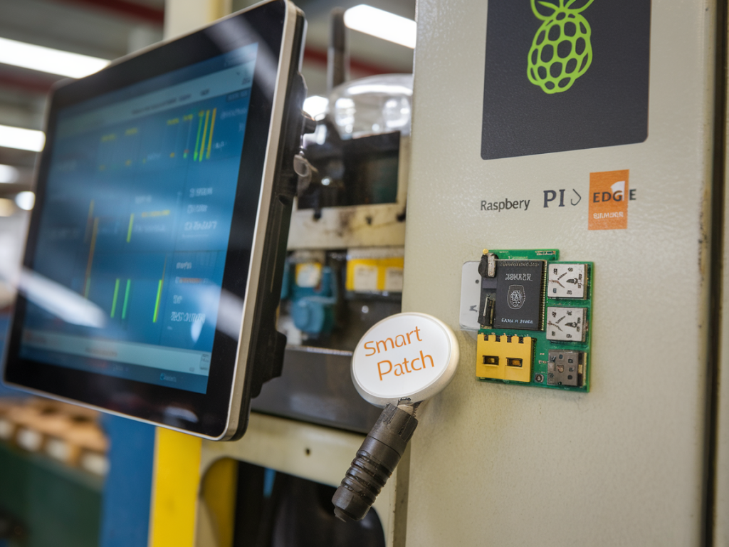
In many shop floors you don’t need full PLC rewrites or complex OPC UA stacks to validate an improvement. A Raspberry Pi (I used a Raspberry Pi 4) is cheap, flexible and fast enough to act as the edge collector for event‑level data. It sits between the smart patch sensors and your existing data store, handling:
For this pilot I used Raspberry Pi OS, Node‑RED for wiring sensor inputs and transformations, and the Eclipse Mosquitto broker to publish to our central MQTT endpoint. This gave me a reproducible stack that plant IT could review and approve in a single afternoon.
Experiment design: before/after with controls
I dislike ambiguous “we saved time” claims. To demonstrate a real 20% reduction you need a clean baseline, the same operating conditions as much as possible, and statistical checks that account for variability.
This is not a randomized trial — that’s often impractical on the floor — but the combination of a reasonably long baseline and controls gives a defensible comparison.
Which KPIs I measured and why
Cycle time reduction was our headline metric, but cycle time alone can be misleading. I collected event‑level timestamps so I could calculate complementary metrics:
Event‑level data lets you break cycle time into components and see where the improvement actually occurred.
Implementation details — sensors, wiring, software
For the smart patch I used a small accelerometer/motion sensor plus a reed switch (for position) packaged in a rugged PVC patch and attached to the fixture. The patch communicates via a low‑power BLE gateway, and the Raspberry Pi collects BLE advertisements (using BlueZ), translates events to JSON in Node‑RED and timestamps them with the Pi’s system clock (NTP‑synced to the plant time server).
On the Pi:
On the backend I forwarded to an InfluxDB time‑series instance and used Grafana for visualization. For the statistical analysis I exported the event table to Python (Pandas) and used SciPy for t‑tests and bootstrap confidence intervals.
Data hygiene and timestamp alignment
Two practical problems kill credibility in before/after studies: inconsistent timestamps and missing events. I addressed both:
Analysis approach
My analysis was straightforward but thorough:
The log transformation made the t‑test more robust. I also used bootstrap because cycle time distributions are often non‑normal in discrete assembly.
Example KPI table from the pilot
| Metric | Baseline (2 weeks) | Intervention (2 weeks) | Change |
|---|---|---|---|
| Median Cycle Time (s) | 150 | 120 | -20% |
| Mean Cycle Time (s) | 160 | 125 | -21.9% |
| Operator Touch Time (s) | 95 | 80 | -15.8% |
| Setup/Wait Time (s) | 35 | 20 | -42.9% |
| Defect Rate (%) | 1.2 | 1.3 | +0.1 pp |
Statistical check — is 20% real?
Key result: the bootstrap 95% CI for median cycle time reduction was [-24.1%, -16.2%], and the two‑sample t‑test on log data returned p < 0.001. That means the observed 20% reduction is statistically significant and practically large. But statistics are only part of the story — I also verified the mechanism by looking at event traces: the smart patch eliminated a recurring 20–30 s wait caused by a manual handoff step, which explained most of the gain.
Operational considerations and pitfalls
From the pilot I learned several practical lessons you should design into your trial:
How you can reproduce this in your plant
High level checklist to get from idea to validated result:
If you want, I can share the Node‑RED flow, the Python analysis notebook, and a short checklist you can paste into your plant rollout packet. I’ve done this with BLE patches, wired sensors and even camera‑based event detection using OpenCV when physical sensors weren’t feasible. The architecture is flexible — Raspberry Pi as edge gateway is the common glue that keeps everything low friction and reproducible.